Introduction to Regression Analysis
Welcome to the comprehensive guide on regression analysis—an indispensable statistical tool used to unravel relationships between variables and make data-driven predictions. In this article, we'll explore the definition, purpose, and historical background of regression analysis, unveiling its transformative impact on various fields of study and decision-making processes.
What is Regression Analysis?
Regression analysis is a statistical method used to examine the relationship between a dependent variable and one or more independent variables. It seeks to identify patterns, correlations, and trends within data and enables researchers and analysts to understand how changes in one variable affect another. The fundamental idea behind regression analysis is to build a model that can predict the values of the dependent variable based on the values of the independent variables.
The Purpose of Regression Analysis
The primary purpose of regression analysis is to extract meaningful insights from data and make informed predictions. By identifying relationships between variables, regression analysis aids in:
- Understanding Dependencies: It helps us comprehend how changes in one variable impact another, providing valuable insights into the nature of relationships.
- Prediction and Forecasting: Regression analysis allows us to predict future outcomes based on historical data, aiding in financial forecasting, market trends, and more.
- Causal Inference: It enables us to determine cause-and-effect relationships, crucial for making evidence-based decisions.
- Optimization and Decision-making: Regression analysis assists in optimizing processes, identifying critical factors, and making data-driven decisions across various domains.
Historical Background and Development
Regression analysis has a rich history, dating back to the early 19th century. The concept can be traced back to the work of Francis Galton, a British polymath, who introduced the idea of "regression to the mean" while studying the inheritance of traits. However, it was the pioneering work of Sir Francis Galton's student, Karl Pearson, that laid the foundation for modern regression analysis.
In the early 20th century, Ronald Fisher made significant contributions to the field, developing the method of least squares, which is widely used in regression analysis today. Subsequently, the field witnessed rapid advancements with the advent of computers, making complex regression models more accessible and applicable across various disciplines.
Understanding Regression Models
The Dependent Variable and Independent Variables
In regression analysis, "The Dependent Variable and Independent Variables" play crucial roles in understanding the relationship between variables and making predictions. Let's delve into the meanings and significance of these terms:
The Dependent Variable:
The dependent variable, often denoted as "Y," is the main outcome or target variable that we seek to predict or explain in regression analysis. It is the variable we are interested in understanding or estimating based on the values of the independent variables. The dependent variable's values are expected to change based on the values of the independent variables, making it the variable we want to model or predict.
For example, in a study examining the relationship between study hours and exam scores, the dependent variable would be the exam scores. The objective is to determine how study hours, the independent variable, influence or affect the dependent variable (exam scores).
Independent Variables:
Independent variables, also known as "predictors" or "explanatory variables," are the variables that may have an impact on the dependent variable. They are denoted as "X₁, X₂, X₃,... Xₙ," and their values are manipulated or observed to understand their influence on the dependent variable. In regression analysis, we assume that changes in the values of the independent variables cause changes in the dependent variable.
Continuing with the previous example, the independent variable would be the study hours. Researchers would gather data on study hours and exam scores from different students to analyze how variations in study hours (independent variable) may lead to changes in exam scores (dependent variable).
Relationship between the Dependent and Independent Variables:
The essence of regression analysis lies in quantifying the relationship between the dependent and independent variables. The goal is to create a mathematical model that best represents the relationship between these variables. This model can then be used to predict the values of the dependent variable based on the values of the independent variables.
The relationship between the dependent and independent variables can be linear or nonlinear, depending on the nature of the data. In simple linear regression, the relationship is represented by a straight line, while in multiple linear regression, it involves a combination of multiple independent variables.
Regression analysis helps us uncover the strength and direction of the relationship between these variables. By understanding how changes in the independent variables impact the dependent variable, we gain valuable insights into the factors influencing the phenomenon under study.
In summary, the dependent variable represents the outcome we want to predict or explain, while the independent variables are the factors we believe may influence the dependent variable. By analyzing the relationship between these variables, regression analysis empowers us to make data-driven predictions and better understand the dynamics of complex systems.
Types of Regression Models
Simple Linear Regression
In statistics, "Simple Linear Regression" is a fundamental and widely used technique to model the relationship between two continuous variables. It aims to establish a linear relationship between a dependent variable and a single independent variable. This allows us to make predictions and understand how changes in the independent variable influence the dependent variable.
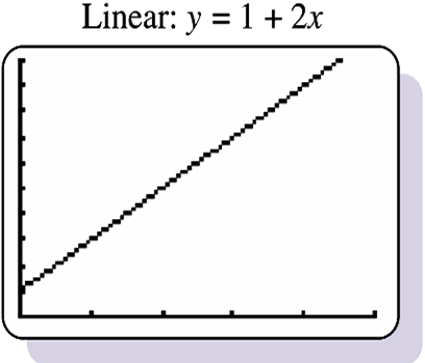
The Equation of Simple Linear Regression:
In simple linear regression, we represent the relationship between the dependent variable (Y) and the independent variable (X) using a straight line equation of the form:
Y = β₀ + β₁X
Where:
- Y represents the dependent variable (also known as the response variable).
- X represents the independent variable (also called the predictor or explanatory variable).
- β₀ is the intercept, representing the value of Y when X is zero.
- β₁ is the slope, indicating the change in Y for a one-unit change in X.
Finding the Best-fitting Line:
The goal of simple linear regression is to find the best-fitting line that minimizes the sum of the squared differences between the observed values of Y and the predicted values from the equation. This line represents the relationship between the variables that best explains the data.
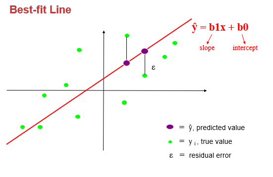
The coefficients β₀ and β₁ are estimated from the data using statistical techniques such as the method of least squares. The method calculates the values of β₀ and β₁ that minimize the sum of the squared residuals (the differences between the observed Y values and the predicted Y values).
Interpreting the Regression Coefficients:
The slope coefficient (β₁) in the simple linear regression equation indicates the change in the dependent variable (Y) for a one-unit change in the independent variable (X). If β₁ is positive, it suggests a positive relationship, meaning that an increase in X is associated with an increase in Y. Conversely, if β₁ is negative, it indicates a negative relationship, where an increase in X corresponds to a decrease in Y.
The intercept coefficient (β₀) represents the value of Y when X is zero. It may or may not have practical significance, depending on the context of the data.
Applications of Simple Linear Regression:
Simple linear regression is widely used in various fields for prediction, forecasting, and understanding relationships between variables. Some common applications include:
- Economics: Studying the relationship between factors like demand and price, income and expenditure, etc.
- Finance: Analyzing the impact of interest rates on investment returns, stock prices, etc.
- Healthcare: Examining the relationship between dosage and drug effectiveness, patient age and recovery time, etc.
- Marketing: Predicting sales based on advertising expenditure, customer engagement, etc.
Limitations of Simple Linear Regression:
While simple linear regression is a powerful tool, it does have limitations. It assumes a linear relationship between the variables, and if the relationship is nonlinear, the model may not be accurate. Additionally, simple linear regression is sensitive to outliers, and it may not be suitable for data with complex relationships.
In conclusion, simple linear regression is a foundational technique in statistics that allows us to model and predict the relationship between two continuous variables using a straight line. It provides valuable insights into the nature of this relationship and finds application in various real-world scenarios across different disciplines.
Multiple Linear Regression
Multiple Linear Regression is an extension of simple linear regression, allowing us to model the relationship between a dependent variable and two or more independent variables. It is a powerful and widely used technique in data analysis, enabling us to understand how multiple factors collectively influence the dependent variable.
The Equation of Multiple Linear Regression:
In multiple linear regression, we represent the relationship between the dependent variable (Y) and multiple independent variables (X₁, X₂, X₃, ... Xₙ) using a linear equation of the form:
Y = β₀ + β₁X₁ + β₂X₂ + β₃X₃ + ... + βₙXₙ
Where:
- Y represents the dependent variable (also known as the response variable).
- X₁, X₂, X₃, ... Xₙ represent the independent variables (also called predictors or explanatory variables).
- β₀ is the intercept, representing the value of Y when all independent variables are zero.
- β₁, β₂, β₃, ... βₙ are the slope coefficients, indicating the change in Y for a one-unit change in each respective independent variable.
Estimating Coefficients:
The coefficients (β₀, β₁, β₂, β₃, ... βₙ) in the multiple linear regression equation are estimated using statistical methods like the method of least squares. The objective is to find the best-fitting line that minimizes the sum of the squared differences between the observed values of Y and the predicted values from the equation.
Estimating the coefficients involves understanding the individual contributions of each independent variable to the dependent variable while considering the presence of other variables in the model.
Interpreting the Regression Coefficients:
In multiple linear regression, each slope coefficient (β₁, β₂, β₃, ... βₙ) represents the change in the dependent variable (Y) for a one-unit change in the corresponding independent variable (X₁, X₂, X₃, ... Xₙ), assuming that all other independent variables remain constant.
The intercept coefficient (β₀) represents the value of Y when all independent variables are zero. However, in practice, this interpretation may not always have practical significance, especially if zero values for all independent variables are not meaningful in the context of the data.
Applications of Multiple Linear Regression:
Multiple linear regression finds extensive applications in various fields due to its ability to incorporate multiple factors in a single model. Some common applications include:
- Economics: Analyzing the impact of multiple economic indicators on a dependent variable, such as GDP, inflation rate, and unemployment rate affecting consumer spending.
- Marketing: Understanding how different marketing strategies, such as advertising expenditure, social media engagement, and product pricing, influence sales.
- Healthcare: Studying how various factors, such as age, gender, lifestyle choices, and medical history, collectively affect a health outcome or disease progression.
- Social Sciences: Exploring the interplay of several socio-economic variables in understanding complex societal issues.
Limitations of Multiple Linear Regression:
Despite its versatility, multiple linear regression has some limitations. It assumes a linear relationship between the dependent and independent variables, and if the relationship is nonlinear, the model may not accurately represent the data. Additionally, multicollinearity, where independent variables are highly correlated, can lead to unstable estimates of coefficients.
In conclusion, multiple linear regression is a powerful statistical technique used to model the relationship between a dependent variable and multiple independent variables. It allows us to analyze the collective impact of various factors on the dependent variable and is widely employed in various fields to gain insights into complex real-world problems.
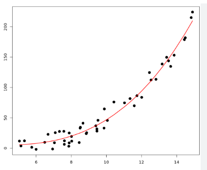
Polynomial Regression
"Polynomial Regression" is a variation of linear regression that accommodates nonlinear relationships between the dependent and independent variables. While simple linear regression assumes a straight-line relationship, polynomial regression allows us to fit a curve to the data points, making it suitable for data that exhibits nonlinear patterns.
The Equation of Polynomial Regression:
In polynomial regression, we represent the relationship between the dependent variable (Y) and the independent variable (X) using a polynomial equation of the form:
Y = β₀ + β₁X + β₂X² + β₃X³ + ... + βₙXⁿ
Where:
- Y represents the dependent variable (also known as the response variable).
- X represents the independent variable (also called the predictor or explanatory variable).
- β₀ is the intercept, representing the value of Y when X is zero.
- β₁, β₂, β₃, ... βₙ are the coefficients of the polynomial terms, determining the shape of the curve.
The polynomial equation allows us to create a curve that fits the data more flexibly, capturing both upward and downward trends in the relationship between the variables.
Choosing the Degree of the Polynomial:
The degree of the polynomial (n) determines the complexity of the curve. It represents the highest power to which X is raised in the equation. For example, a polynomial of degree 2 (quadratic) would have terms like X², while a polynomial of degree 3 (cubic) would have terms like X³.
Choosing the appropriate degree of the polynomial is crucial as an overly complex model may lead to overfitting, where the model fits the noise in the data rather than the underlying pattern. On the other hand, a too simple model may not capture the true relationship adequately.
Applications of Polynomial Regression:
Polynomial regression finds application in scenarios where the data does not follow a linear trend but exhibits a more curvilinear pattern. Some common applications include:
- Growth Analysis: Modeling the growth of organisms or populations over time, where the rate of growth may not be linear.
- Engineering and Physics: Understanding the relationship between physical variables, such as force and displacement, temperature and pressure, etc.
- Finance: Analyzing the impact of compounding interest or inflation on investments.
- Climate Studies: Studying temperature changes over time, where the relationship may not be linear due to various factors.
Limitations of Polynomial Regression:
While polynomial regression can capture complex relationships, it has some limitations. As the degree of the polynomial increases, the model becomes more complex, leading to potential overfitting. Additionally, polynomial regression may not be suitable for extrapolation beyond the range of observed data, as the curve may behave erratically outside the data range.
Careful consideration of the data and degree selection is essential to ensure the model's accuracy and generalization to new data points.
In conclusion, polynomial regression is a valuable extension of linear regression, allowing us to model nonlinear relationships between variables. By introducing polynomial terms, the model can fit curves to the data, enabling more flexible and accurate predictions in scenarios where linear relationships are insufficient.
Logistic Regression
I. Introduction to Logistic Regression
A. Understanding Binary Classification
Logistic regression is a powerful statistical method used for binary classification tasks, where the outcome variable can take only two possible values, usually denoted as 0 and 1. The goal is to predict the probability of an event belonging to a particular category based on one or more independent variables.
In binary classification scenarios, we seek answers to questions like:
- Will a customer churn or stay with a subscription service?
- Does a patient have a particular disease or not?
- Will a credit card transaction be fraudulent or legitimate?
Logistic regression allows us to make informed decisions by calculating the probability of an event's occurrence.
B. Real-world Applications
The versatility of logistic regression makes it applicable across various domains:
- Healthcare: Predicting disease outcomes, diagnosing medical conditions.
- Finance: Assessing credit risk, detecting fraudulent transactions.
- Marketing: Identifying potential customers, targeting ads effectively.
- Social Sciences: Analyzing survey responses, predicting voting behavior.
II. The Logistic Regression Model
A. The Sigmoid Function
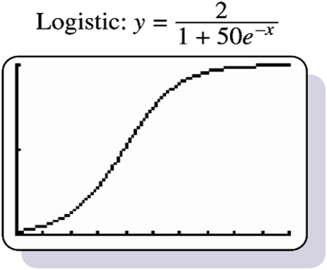
The fundamental principle behind logistic regression lies in the use of the sigmoid function, which maps any real-valued number to a value between 0 and 1. The sigmoid function is defined as:
p = 1 / (1 + e^(-z))
Where:
- p is the probability of the event being 1 (success).
- e is the base of the natural logarithm (approximately 2.71828).
- z is the linear combination of the independent variables and their coefficients.
The sigmoid function ensures that the probability is bounded within the range [0, 1], making it suitable for binary classification.
B. Coefficients and Log-Odds
The logistic regression model estimates coefficients (β₀, β₁, β₂, ... βₙ) for each independent variable, representing the impact of these variables on the log-odds of the event being 1. The log-odds, also known as the logit, is the logarithm of the odds ratio, which measures the likelihood of an event occurring.
The linear combination (z) of the independent variables and coefficients is given by:
z = β₀ + β₁X₁ + β₂X₂ + ... + βₙXₙ
C. Decision Threshold
To classify the outcome into either 0 or 1, a decision threshold is chosen (commonly 0.5). If the predicted probability (p) is equal to or greater than the threshold, the event is classified as 1; otherwise, it is classified as 0.
III. Data Preparation for Logistic Regression
A. Collecting and Organizing Data
Data preparation is crucial for successful logistic regression. Ensure that you have collected relevant data with the dependent variable and independent variables. Organize the data into a structured format suitable for analysis.
B. Handling Missing Values
Address any missing values in the dataset. Impute or remove missing values as appropriate to maintain the integrity of the analysis.
C. Feature Scaling and Normalization
For better model convergence and interpretability, consider scaling and normalizing the independent variables. This step is especially essential when dealing with variables of different scales.
IV. Model Building and Evaluation
A. Splitting the Data into Training and Test Sets
Before fitting the logistic regression model, split the data into training and test sets. The training set is used to build the model, while the test set is used to evaluate its performance on unseen data.
B. Fitting the Logistic Regression Model
Using the training data, fit the logistic regression model. The model will estimate the coefficients for the independent variables.
C. Evaluating Model Performance
Evaluate the model's performance using metrics such as accuracy, precision, recall, and F1 score. Adjust the model as needed to improve its predictive capabilities.
Applications of Logistic Regression
Logistic regression finds applications in various real-world scenarios due to its versatility and interpretability.
A. Medical Diagnostics
In medical diagnostics, logistic regression can predict the likelihood of a patient having a particular disease based on medical history, symptoms, and test results. It aids in early detection and timely treatment.
B. Customer Churn Prediction
Businesses use logistic regression to predict customer churn and take proactive measures to retain valuable customers. It helps identify factors leading to customer attrition.
C. Credit Risk Analysis
In the financial sector, logistic regression assesses credit risk by predicting the likelihood of default based on customers' credit history and financial profiles.
D. Marketing and Sales
Logistic regression assists in targeting marketing efforts by predicting the likelihood of a customer making a purchase. It optimizes marketing campaigns and resource allocation.
Advantages and Limitations of Logistic Regression
A. Simplicity and Interpretability
Logistic regression is easy to implement and interpret, making it a popular choice for initial modeling and inference.
B. Handling Nonlinear Relationships
While logistic regression is excellent for linear relationships, it may not capture complex nonlinear relationships present in the data.
C. Sensitivity to Outliers and Multicollinearity
Logistic regression can be sensitive to outliers and multicollinearity, which may impact the model's performance.
Real-life Examples of Logistic Regression Projects
A. Predicting Loan Default
In a loan default prediction project, logistic regression helps financial institutions assess the likelihood of a borrower defaulting based on historical loan data.
B. Detecting Fraudulent Transactions
Logistic regression assists in identifying fraudulent transactions by analyzing transaction patterns and customer behavior.
C. Identifying Disease Risk Factors
In medical research, logistic regression helps identify risk factors associated with diseases, guiding public health initiatives and preventive measures.
In summary, logistic regression is a powerful tool for binary classification tasks, providing probabilities for class membership based on independent variables. It is widely used in diverse applications and allows us to make informed decisions by understanding the relationships between variables and predicting binary outcomes.
Advancements and Future Trends in Regression Models
The Evolution of Regression Models
Regression analysis has been a fundamental statistical tool for centuries, helping us understand relationships between variables and make predictions. Over time, it has evolved to address complex real-world problems in diverse fields such as finance, healthcare, and marketing.
The Importance of Advancements in Regression Analysis
As the volume and complexity of data increase, the need for more sophisticated regression models becomes evident. Advancements in technology, the availability of vast datasets, and the integration of machine learning techniques have opened new horizons for regression analysis. This article explores these advancements and future trends shaping the field of regression models.
Integration of Machine Learning Techniques
A. Overview of Machine Learning
Machine learning is a subset of artificial intelligence (AI) that focuses on enabling systems to learn from data and improve their performance over time without explicit programming. It encompasses a range of algorithms that can learn patterns and relationships from data, making it an ideal complement to traditional regression models.
B. How Machine Learning Enhances Regression Models
The integration of machine learning techniques, such as decision trees, random forests, and support vector machines, has revolutionized regression analysis. These algorithms can capture complex patterns and nonlinear relationships that traditional linear regression may miss.
C. Use Cases and Examples
Machine learning-enhanced regression models find applications in predictive analytics, time-series forecasting, and anomaly detection. For example, in healthcare, machine learning regression models can predict disease outcomes based on patient data, leading to personalized treatment plans.
Big Data and its Impact on Regression Models
A. Understanding Big Data and its Challenges
The era of big data has transformed the way organizations handle information. Big data refers to massive datasets that traditional data processing methods may struggle to analyze. Challenges include data storage, processing speed, and data quality.
B. Scalability and Efficiency in Regression Analysis
Regression models must adapt to handle large datasets efficiently. Modern tools and techniques allow regression analysis to scale and process big data effectively, making it feasible to extract valuable insights from vast information pools.
C. Realizing Insights from Massive Datasets
By incorporating big data into regression models, businesses gain a competitive advantage. Retailers can analyze customer behavior from vast transaction histories, while financial institutions can identify patterns in market data for better investment decisions.
Hybrid Models and Ensemble Techniques
A. Introduction to Hybrid Models
Hybrid models combine multiple regression techniques or integrate regression with other algorithms to overcome limitations and enhance accuracy. These models are particularly useful when datasets exhibit complex relationships.
B. Combining Regression with Other Algorithms
Hybrid models leverage the strengths of different algorithms to create a more robust and comprehensive model. For instance, combining linear regression with decision trees can lead to better predictions in scenarios with both linear and nonlinear relationships.
C. Ensemble Techniques for Improved Accuracy
Ensemble techniques, such as bagging and boosting, aggregate the predictions of multiple regression models to achieve higher accuracy. These methods reduce overfitting and improve generalization capabilities.
The Future of Regression Models
A. Incorporating AI and Automation
The future of regression analysis lies in harnessing the power of AI and automation. Automation tools can streamline the model-building process, allowing analysts to focus on interpreting results and deriving actionable insights.
B. Explainable AI and Interpretability
As AI integration becomes more prevalent, the need for explainable AI becomes paramount. Transparent models that provide clear explanations for predictions ensure trust and acceptance in critical decision-making processes.
C. Addressing Biases and Ethical Considerations
With the increasing reliance on regression models for decision-making, it is essential to address biases in data and models to avoid discriminatory outcomes. Ethical considerations must be at the forefront of regression analysis.
Practical Applications and Success Stories
A. Predictive Analytics in Healthcare
Regression models help predict patient outcomes and assist in diagnosing diseases. For example, predictive models can forecast the likelihood of readmissions for certain patients, leading to improved healthcare interventions.
B. Financial Forecasting and Risk Management
Regression models play a crucial role in financial forecasting, such as predicting stock prices or estimating default probabilities for loans. Risk management relies on regression analysis to identify potential financial risks.
C. Marketing and Customer Behavior Analysis
Marketers use regression models to understand customer behavior and preferences. Analyzing past data helps create targeted marketing campaigns, leading to higher conversion rates.
Challenges and Limitations
A. Overfitting and Model Complexity
Complex regression models can be susceptible to overfitting, where the model performs well on the training data but poorly on unseen data. Careful model selection and validation are necessary to mitigate overfitting.
B. Data Quality and Feature Engineering
Regression models heavily rely on the quality and relevance of the input data. Proper feature engineering is essential to ensure meaningful results and accurate predictions.
C. Interpreting Nonlinear Relationships
Traditional regression models struggle to capture nonlinear relationships between variables. As datasets become more complex, addressing nonlinearity becomes a significant challenge.
Conclusion
Advancements in regression models have expanded their capabilities, making them indispensable tools for data analysis and decision-making. Integration with machine learning, utilization of big data, and hybrid models contribute to better predictions and insights.
As businesses continue to embrace data-driven decision-making, regression models will remain crucial for uncovering meaningful patterns and relationships within the data. Leveraging these models ensures organizations stay competitive and make informed choices.
Frequently Asked Questions (FAQs)
Q: What is the purpose of regression analysis?
A: The purpose of regression analysis is to examine the relationship between a dependent variable and one or more independent variables. It aims to model the functional relationship between these variables to make predictions and understand how changes in the independent variables affect the dependent variable. Regression analysis is commonly used for forecasting, estimating trends, and identifying patterns in data.
Q: How are dependent and independent variables related in regression models?
A: In regression models, the dependent variable (also known as the response variable) is the outcome of interest, and the independent variables (also known as predictor variables) are the variables used to predict or explain the dependent variable. The regression model estimates the coefficients of the independent variables, which represent the change in the dependent variable for a unit change in each independent variable, while holding other variables constant.
Q: What are the key differences between simple linear and multiple linear regression?
A: The key differences between simple linear and multiple linear regression are as follows:
- Number of Independent Variables:
- Simple Linear Regression: It involves only one independent variable.
- Multiple Linear Regression: It involves two or more independent variables.
- Model Equation:
- Simple Linear Regression: The model equation is of the form Y = β₀ + β₁X, where Y is the dependent variable, X is the independent variable, β₀ is the intercept, and β₁ is the slope coefficient.
- Multiple Linear Regression: The model equation is of the form Y = β₀ + β₁X₁ + β₂X₂ + ... + βₙXₙ, where Y is the dependent variable, X₁, X₂, ..., Xₙ are the independent variables, and β₀, β₁, β₂, ..., βₙ are the coefficients.
- Complexity and Interpretability:
- Simple Linear Regression: It is relatively simpler and easier to interpret since it involves only one independent variable.
- Multiple Linear Regression: It is more complex and may require additional statistical techniques for interpretation due to multiple independent variables.
Q: When is polynomial regression more suitable than other models?
A: Polynomial regression is more suitable than other models when the relationship between the dependent and independent variables is nonlinear. In cases where the data points do not follow a straight-line pattern, polynomial regression allows the model to capture curvature and flexibility. It involves fitting a polynomial function to the data, enabling better representation of complex relationships. However, it is essential to use polynomial regression judiciously, as higher-degree polynomials can lead to overfitting if not carefully controlled.
Q: How does logistic regression handle binary outcomes?
A: Logistic regression handles binary outcomes by using the logistic (sigmoid) function to map the linear combination of independent variables and their coefficients to a value between 0 and 1. The logistic function ensures that the predicted probability lies within the range [0, 1], making it suitable for binary classification tasks. If the predicted probability is greater than or equal to a predefined decision threshold (often 0.5), the observation is classified as belonging to the positive class (1); otherwise, it is classified as belonging to the negative class (0). Logistic regression is widely used for binary classification problems, such as predicting the probability of an event occurring or not occurring based on the given features.