Hypothesis Testing 101 – What is at the “heart” of hypothesis testing in statistics?

Hypothesis testing is a fundamental statistical technique used to make inferences and draw conclusions about a population based on sample data. It allows researchers to evaluate the validity of a claim or hypothesis by analyzing the evidence present in the data. In this blog post, we will delve into the intricacies of hypothesis testing, exploring its concepts, data reconfigurations, terminologies, and various types of hypothesis tests along with their real-world applications.

1. Understanding Hypothesis Testing

Definition and Purpose

Hypothesis testing is a statistical method used to assess the validity of a claim or hypothesis about a population based on sample data. It involves formulating a null hypothesis (H0 - pronounced as "H-Nought") and an alternative hypothesis (Ha), collecting and analyzing data, and making a decision regarding the acceptance or rejection of the null hypothesis.

In statistical terms, Hypothesis Testing can help establish a statistical difference between factors from different distributions.

2. Key Concepts in Hypothesis Testing

Hypothesis Testing begins with defining the objective and scope of the study. The key step is to define the assumptions or the hypotheses for the target study (that is, Null and Alternate Hypothesis)

Null Hypothesis (H0)

The null hypothesis is a statement of no effect or no difference. It assumes that any observed difference or effect is due to random chance or sampling variability.

Alternative Hypothesis (Ha)

The alternative hypothesis is a statement that contradicts the null hypothesis. It suggests that there is a significant effect or difference present in the population.

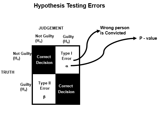
The concept of hypothesis testing can very well be illustrated by the example of a "criminal trial" in a court of law. A person accused of a crime has to face a trial where the prosecution presents the evidence against the person to convict him/her. The jury or the judge has to make a decision based on the evidence presented by the prosecution or the defense. The judge or the jury is only conducting the hypothesis test in the trial process. The "null hypothesis" is that the person is innocent and the "Alternate hypothesis" is that the person is guilty.

There are two possible decisions - either the person is convicted or set free. Conviction means that the jury decided to reject Null hypothesis, while acquitting means not rejecting the null hypothesis

There are two possible types of error in this decision making process of Hypothesis Testing:

Type I Error (Alpha)

A Type I error occurs while the null hypothesis is rejected, even when it is, in fact, true. It represents a false positive or a false rejection of a true null hypothesis. In trial example, Type I error occurs when the innocent person is wrongly convicted.

Type II Error (Beta)

A Type II error occurs while the null hypothesis is not rejected, when it is, in fact, false. It represents a false negative or a failure to reject a false null hypothesis. In trial example, Type II error occurs when the guilty person is wrongly acquitted.

Significance Level (Alpha Level)

The significance level, often denoted as alpha (α), is the threshold set for rejecting the null hypothesis. It represents the maximum probability of committing a Type I error. Normally it is set at 0.05.

P-Value

The p-value is the probability of obtaining a test statistic as extreme as the one observed or more extreme, assuming that the null hypothesis is true. It helps in deciding whether to reject or fail to reject the null hypothesis.

If P-value < 0.05, Reject H0,    which means there is a difference or relationship

If P-value > 0.05, fail to reject H0, which means there is no difference or relationship

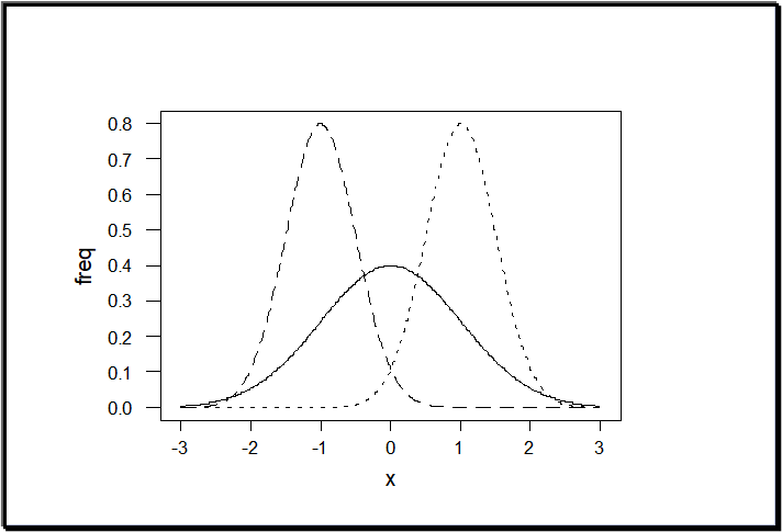
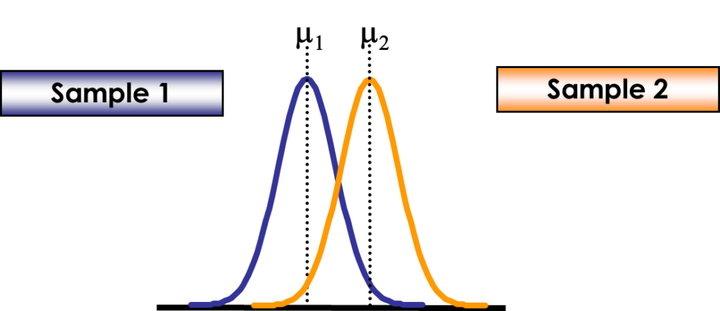
Critical Region

The critical region is the range of values for the test statistic that leads to the rejection of the null hypothesis. It is determined by the significance level and the nature of the test.

In above illustration, orange distribution is the population distribution and the blue distribution above is the sample distribution for which the p-value is calculated. If the p-value falls in the "Rejection Region", then the H0 is rejected which means there is no statistically significant difference between the population and sample distribution attributes.

3. Types of Hypothesis Tests

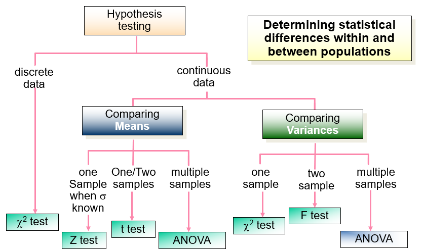
3.1 One-Sample T-Test

One commonly used hypothesis test is the one sample t-test. The one-sample t-test is used to determine whether the mean of a sample differs significantly from a known or hypothesized population mean.

Understanding the One Sample T-Test

The one sample t-test is used to determine whether the mean of a sample significantly differs from a known population mean. It helps us investigate whether the observed sample mean is significantly different from what we would expect by chance.

Assumptions of the One Sample T-Test

Before conducting a one sample t-test, it is important to ensure that certain assumptions are met. These assumptions include:

1. Random Sampling: The sample should be randomly selected from the population of interest.
2. Independence: The observations within the sample should be independent of each other.
3. Normality: The data should follow a normal distribution within the population.
4. Homogeneity of Variance: The variances of the population and sample should be equal.

Conducting a One Sample T-Test

To perform a one sample t-test, follow these steps:

1. State the null and alternative hypotheses.
2. Select an appropriate significance level (e.g., 0.05).
3. Collect sample data and calculate the sample mean and standard deviation.
4. Determine the critical t-value or p-value based on the chosen significance level and degrees of freedom.
5. Calculate the test statistic, which is the t-value.

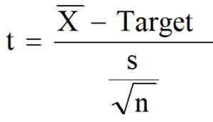
t = t test statistic

Target is the hypothesized mean of the population

s = Standard deviation of the sample

n = sample size

6. Compare the test statistic with the critical value or p-value.

7. Make a decision to either reject or fail to reject the null hypothesis based on the comparison.

Interpreting the Results

After conducting a one sample t-test, interpreting the results is crucial. If the p-value is less than the chosen significance level, typically 0.05, we reject the null hypothesis. This suggests that there is a significant difference between the sample mean and the known population mean. On the other hand, if the p-value is greater than the significance level, we fail to reject the null hypothesis, indicating that there is no significant difference.

3.2 Two-Sample T-Test

A two-sample t-test, also known as an independent samples t-test, compares the means of two independent groups to determine if they are significantly different from each other. It is commonly used when comparing the means of two treatment groups, two populations, or two different conditions.

Assumptions of the Two-Sample T-Test

Before conducting a two-sample t-test, certain assumptions must be met. These assumptions include:

1. Independence: The observations within each group should be independent of each other.
2. Normality: The data within each group should follow a normal distribution.
3. Equal Variances: The variances of the two groups should be equal. If the variances are not equal, a modified version of the t-test called Welch's t-test can be used.

Conducting a Two-Sample T-Test

To perform a two-sample t-test, follow these steps:

1. State the null and alternative hypotheses.
2. Select an appropriate significance level (e.g., 0.05).
3. Collect data from the two independent groups.
4. Calculate the sample means and standard deviations for each group.
5. Determine the critical t-value or p-value based on the chosen significance level and degrees of freedom.
6. Calculate the test statistic, which is the t-value.
   • The formula for calculating the t-statistic in a two-sample t-test is as follows:
   • t = (x1 - x2) / sqrt((s1^2 / n1) + (s2^2 / n2))
     • Where:
     • x1 and x2 are the sample means of the two independent groups.
     • s1 and s2 are the sample standard deviations of the two groups.
     • n1 and n2 are the sample sizes of the two groups.
7. Compare the test statistic with the critical value or p-value.
8. Make a decision to either reject or fail to reject the null hypothesis based on the comparison.

Interpreting the Results

After conducting a two-sample t-test, interpreting the results is essential. If the p-value is less than the chosen significance level, typically 0.05, we reject the null hypothesis. This suggests that there is a significant difference between the means of the two groups. Conversely, if the p-value is greater than the significance level, we fail to reject the null hypothesis, indicating that there is no significant difference.

3.3 Paired T-Test

The paired t-test is used to determine if there is a significant difference between the means of two related groups. It is specifically designed to analyze situations where each observation in one group is matched or paired with a corresponding observation in the other group. This could be the case when measuring the same individuals before and after an intervention, or when comparing results from two different techniques applied to the same subjects.

Assumptions of the Paired t-test

Before conducting a paired t-test, certain assumptions must be met. These assumptions include:

1. Dependence: The two groups being compared should consist of paired or dependent observations.
2. Normality: The differences between the paired observations should follow a normal distribution.
3. Independence: The paired differences should be independent of each other.

Conducting a Paired t-test

To perform a paired t-test, follow these steps:

1. State the null and alternative hypotheses.
2. Select an appropriate significance level (e.g., 0.05).
3. Collect paired data from the related groups.
4. Calculate the differences between the paired observations.
5. Calculate the sample mean and standard deviation of the differences.
6. Determine the critical t-value or p-value based on the chosen significance level and degrees of freedom.
7. Calculate the test statistic, which is the t-value.
8. Compare the test statistic with the critical value or p-value.
9. Make a decision to either reject or fail to reject the null hypothesis based on the comparison.

Interpreting the Results

After conducting a paired t-test, interpreting the results is crucial. If the p-value is less than the chosen significance level, typically 0.05, we reject the null hypothesis. This suggests that there is a significant difference between the means of the paired groups. Conversely, if the p-value is greater than the significance level, we fail to reject the null hypothesis, indicating that there is no significant difference.

3.4 Z-Test

A Z-test is a statistical test used to determine whether there is a significant difference between a sample mean and a known population mean when the population standard deviation is known. It is based on the standard normal distribution, where the Z-score measures the number of standard deviations a data point is from the mean.

When to Use a Z-Test

The Z-test is appropriate under the following conditions:

• The sample size is large (typically n > 30).
• The population standard deviation is known.
• The data are normally distributed or follow the Central Limit Theorem.

Assumptions of the Z-Test

Before conducting a Z-test, certain assumptions must be met, including:

1. Random Sampling: The sample should be randomly selected from the population of interest.
2. Independence: The observations within the sample should be independent of each other.
3. Normality: The data should follow a normal distribution or approximately normal due to the Central Limit Theorem.
4. Population Standard Deviation: The population standard deviation should be known.

Conducting a Z-Test

To perform a Z-test, follow these steps:

1. State the null and alternative hypotheses.
2. Select an appropriate significance level (e.g., 0.05).
3. Collect sample data and calculate the sample mean.
4. Determine the critical Z-value based on the chosen significance level.
5. Calculate the test statistic, which is the Z-score.
   • The test statistic is => Z = (xbar – μ0) / (σ/√n)
   • Where, xbar = Sample mean
   • μ0 = Population Mean / Hypothesized mean
   • σ = Population Standard Deviation
   • n = Sample mean
6. Compare the test statistic with the critical value.
7. Make a decision to either reject or fail to reject the null hypothesis based on the comparison.

Interpreting the Results

After conducting a Z-test, interpreting the results is crucial. If the test statistic falls within the critical region (beyond the critical value), the null hypothesis is rejected, suggesting a significant difference between the sample mean and the known population mean. Conversely, if the test statistic falls within the non-critical region, the null hypothesis is not rejected, indicating no significant difference.

3.5 Chi-Square Test

The Chi-Square test is a powerful tool that allows us to analyze categorical data and determine if there is a significant association or difference between variables. In this article, we will explore the Chi-Square test, its types, assumptions, how to conduct the test, interpret the results, and its real-world applications. Understanding the Chi-Square test is crucial for researchers and data analysts dealing with categorical data.

What is a Chi-Square Test?

A Chi-Square test is a statistical test used to determine the association or independence between two categorical variables. It compares the observed frequencies of categories with the expected frequencies under a null hypothesis of independence. The test produces a Chi-Square statistic and a p-value, which help assess the significance of the relationship between variables.

Types of Chi-Square Tests

There are two main types of Chi-Square tests:

1. Chi-Square Test of Independence: This test examines whether two categorical variables are independent of each other.
2. Chi-Square Goodness-of-Fit Test: This test determines if an observed frequency distribution fits an expected theoretical distribution.

Assumptions of the Chi-Square Test

Before conducting a Chi-Square test, certain assumptions should be considered:

1. Independence: The observations should be independent and come from a random sample.
2. Sample Size: The sample size should be sufficiently large for the Chi-Square distribution to be applicable.
3. Expected Cell Frequencies: The expected cell frequencies should not be too small (usually greater than 5) to ensure the validity of the test.

Conducting a Chi-Square Test

To perform a Chi-Square test, follow these steps:

1. State the null and alternative hypotheses.
2. Select an appropriate significance level (e.g., 0.05).
3. Organize the data into a contingency table.
4. Calculate the expected frequencies for each cell of the table.
5. Calculate the Chi-Square test statistic based on the observed and expected frequencies.
6. Determine the degrees of freedom for the test.
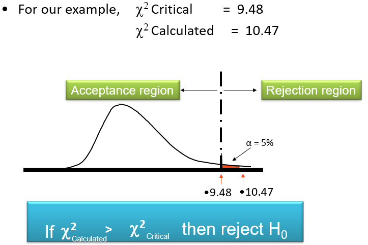
7. Compare the calculated Chi-Square statistic with the critical Chi-Square value or calculate the p-value.
   • The Chi-Square statistic is calculated by:

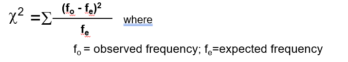
8. Make a decision to either reject or fail to reject the null hypothesis based on the comparison.

Interpreting the Results

After conducting a Chi-Square test, interpreting the results is crucial. If the p-value is less than the chosen significance level (e.g., 0.05), we reject the null hypothesis. This indicates that there is evidence of a significant association or difference between the categorical variables. Conversely, if the p-value is greater than the significance level, we fail to reject the null hypothesis, suggesting no significant association.

3.6 ANOVA (Analysis of Variance)

ANOVA, or Analysis of Variance, is a statistical method used to compare the means of two or more groups. It helps determine whether the observed differences between group means are statistically significant or simply due to chance. ANOVA analyzes the variation within and between groups to assess the significance of group differences.

One-Way ANOVA

One-Way ANOVA is used when there is one categorical independent variable and a continuous dependent variable. It tests whether the means of the dependent variable are significantly different across the levels of the independent variable. One-Way ANOVA allows for comparisons among multiple groups.

Two-Way ANOVA

Two-Way ANOVA extends the analysis to include two independent variables, allowing for the examination of interactions between them. It assesses the influence of each independent variable individually as well as their combined effects on the dependent variable. Two-Way ANOVA provides insights into group differences and interaction effects.

Assumptions of ANOVA

Before conducting an ANOVA analysis, several assumptions must be considered:

1. Independence: Observations within each group and between groups should be independent of each other.
2. Normality: The dependent variable should follow a normal distribution within each group.
3. Homogeneity of Variance: The variances of the dependent variable should be approximately equal across all groups.

Conducting an ANOVA Analysis

To perform an ANOVA analysis, follow these steps:

1. State the null and alternative hypotheses.
2. Select an appropriate significance level (e.g., 0.05).
3. Collect data and organize it into groups based on the categorical independent variable.
4. Calculate descriptive statistics for each group, including means and standard deviations.
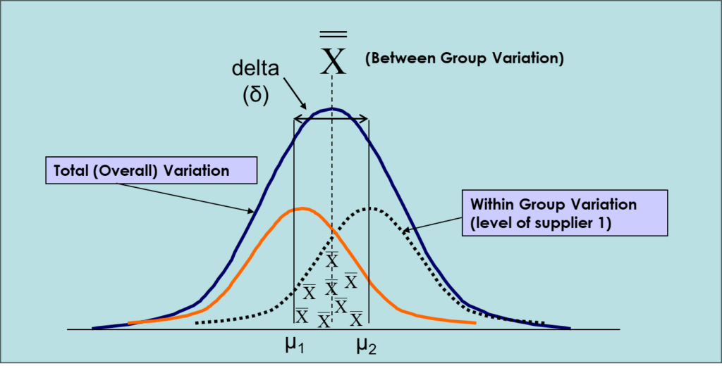
5. Conduct an ANOVA test to calculate the F-statistic and p-value.
   • F-Statistic = Between Group variance/ Within group variance
6. Determine the degrees of freedom for the analysis.
7. Compare the p-value with the chosen significance level.
8. Make a decision to either reject or fail to reject the null hypothesis based on the p-value.

Interpreting the Results

After conducting an ANOVA analysis, interpreting the results is essential. If the p-value is less than the chosen significance level, the null hypothesis is rejected, indicating that there are significant differences between at least two groups. On the other hand, if the p-value is greater than the significance level, the null hypothesis is not rejected, suggesting no significant differences among the groups.

Advantages and Limitations of ANOVA

ANOVA offers several advantages, including:

• It allows for the comparison of means across multiple groups.
• It provides information about the significance of group differences.

However, there are limitations to consider:

• ANOVA assumes independence, normality, and homogeneity of variance.
• It may not be suitable for small sample sizes or non-parametric data.

Real-World Applications

ANOVA has numerous applications across various fields, including:

• Biomedical research: Comparing the efficacy of different treatments on patient outcomes.
• Education: Assessing the impact of different teaching methods on student performance.
• Market research: Analyzing consumer preferences across different demographic groups.

3.7 Non parametric tests

Nonparametric tests, also known as distribution-free tests, are statistical methods used to analyze data when the underlying population distribution is unknown or does not follow a specific distribution. These tests are valuable in situations where the assumptions of parametric tests, such as normality and equal variances, are not met. Nonparametric tests provide alternative approaches that rely on fewer assumptions, making them more robust and flexible.

Unlike parametric tests that make assumptions about the shape and parameters of the population distribution, nonparametric tests focus on the ranks or order of the data rather than the actual values. This characteristic allows them to be applied to a wide range of data types, including ordinal, interval, and nominal variables. Nonparametric tests are particularly useful when dealing with small sample sizes, skewed distributions, outliers, or non-normal data.

Nonparametric tests, also known as distribution-free tests, are statistical methods used to analyze data when the underlying population distribution is unknown or does not follow a specific distribution. These tests are valuable in situations where the assumptions of parametric tests, such as normality and equal variances, are not met. Nonparametric tests provide alternative approaches that rely on fewer assumptions, making them more robust and flexible.

Unlike parametric tests that make assumptions about the shape and parameters of the population distribution, nonparametric tests focus on the ranks or order of the data rather than the actual values. This characteristic allows them to be applied to a wide range of data types, including ordinal, interval, and nominal variables. Nonparametric tests are particularly useful when dealing with small sample sizes, skewed distributions, outliers, or non-normal data.

Here are some commonly used nonparametric tests:

1. Mann-Whitney U test: This test is used to compare the medians of two independent groups. It assesses whether there is a statistically significant difference between the distributions of the two groups.
2. Wilcoxon signed-rank test: This test is used to compare the medians of two related or paired samples. It evaluates whether there is a significant difference between the two measurements taken on the same individuals.
3. Kruskal-Wallis test: This test is an extension of the Mann-Whitney U test and is used to compare the medians of three or more independent groups. It determines if there are significant differences among the groups.
4. Friedman test: This test is similar to the Kruskal-Wallis test but is applied to repeated measures or matched samples. It compares the medians of three or more related groups.
5. Chi-Square test: The Chi-Square test is used to analyze categorical data. It determines whether there is a significant association or difference between two or more categorical variables.
6. Runs test: This test examines whether a sequence of observations is random or exhibits a systematic pattern.
7. Sign test: The sign test is used to analyze paired data and determines if there is a significant difference between two measurements.

5. Real-World Applications of Hypothesis Testing

Medical Research and Clinical Trials

Hypothesis testing plays a crucial role in medical research and clinical trials, helping to evaluate the effectiveness of new treatments, compare the outcomes of different interventions, and assess the safety of medications.

Quality Control and Six Sigma

In manufacturing and quality control processes, hypothesis testing is used to ensure product quality, identify process improvements, and measure the impact of process changes.

Market Research and Surveys

Hypothesis testing is employed in market research and surveys to analyze consumer behavior, test marketing strategies, evaluate advertising campaigns, and validate research hypotheses.

Social Sciences and Psychology

Researchers in social sciences and psychology use hypothesis testing to study human behavior, investigate the effectiveness of interventions, and explore relationships between variables.

Environmental Studies

Hypothesis testing aids environmental scientists in analyzing the impact of pollution, climate change, and other factors on ecosystems, biodiversity, and natural resources.

Business and Finance

In business and finance, hypothesis testing is utilized to make informed decisions, assess investment strategies, analyze financial data, and evaluate the performance of financial models.

6. Conclusion

In conclusion, hypothesis testing is a powerful statistical tool that allows researchers to draw meaningful conclusions based on sample data. By formulating clear hypotheses, selecting appropriate tests, and interpreting the results correctly, one can make well-informed decisions in various fields, ranging from scientific research to business analytics. Understanding the concepts, terminologies, and various types of hypothesis tests is essential for conducting rigorous analyses and advancing knowledge in diverse domains.

Frequently Asked Questions (FAQs)

1. What is the purpose of hypothesis testing?
   • Hypothesis testing is used to evaluate the validity of a claim or hypothesis about a population based on sample data.
2. How many types of hypothesis tests are there?
   • There are several types of hypothesis tests, including one-sample t-test, two-sample t-test, chi-square test, ANOVA, z-test, and many more.
3. What is a p-value, and how is it used in hypothesis testing?
   • The p-value is the probability of obtaining a test statistic as extreme as the one observed, assuming that the null hypothesis is true. It helps in deciding whether to reject or fail to reject the null hypothesis.
4. What are Type I and Type II errors?
   • Type I error occurs when the null hypothesis is rejected, but it is true. Type II error occurs when the null hypothesis is not rejected, but it is false.
5. How is hypothesis testing applied in real-world scenarios?
   • Hypothesis testing finds applications in medical research, quality control, market research, social sciences, environmental studies, and business analytics, among others.
6. What role does the Central Limit Theorem play in hypothesis testing? The CLT is used to create a null distribution against which the observed sample mean can be compared. This helps determine the statistical significance of the results.