How to do Model Performance Evaluation in Machine Learning :- Key Methodologies

Definition of Model Performance Evaluation

Model Performance Evaluation is a critical process in the field of machine learning, aimed at assessing the effectiveness and accuracy of a trained predictive model. It involves comparing the model's predictions against the actual outcomes or ground truth data to determine how well the model performs on unseen data in future. The primary goal of model evaluation is to understand the model's strengths, weaknesses, and potential areas for improvement.

In simpler terms, when we build a machine learning model to make predictions, we want to know how reliable and accurate those predictions are. Model Performance Evaluation helps us answer questions like: How often does the model make correct predictions (accuracy of the model)? Is the model biased towards a particular class or outcome? Does the model generalize well to new data?

The process of evaluating model performance goes beyond just looking at the accuracy or error rate. It involves a thorough analysis of various performance metrics, such as precision, recall, F1 Score, ROC Curve, AUC, and more. Each of these metrics provides different insights into the model's behavior and can be useful in different scenarios.

Model Performance Evaluation also involves the use of cross-validation techniques to get a more reliable estimate of the model's performance on unseen data. By dividing the dataset into multiple subsets and training the model on different combinations of these subsets, we can assess how well the model generalizes to new data and detect potential issues like overfitting.

Moreover, model evaluation is an iterative process that continues even after the model has been deployed in real-world applications. Continuous monitoring of the model's performance is essential to detect model drift, which occurs when the model's accuracy deteriorates over time due to changes in the data distribution or other external factors. By monitoring model performance, data scientists can take timely actions to retrain or fine-tune the model to maintain its accuracy and relevance.

Importance of Model Performance Evaluation in Machine Learning

Model Evaluation holds immense significance in the realm of machine learning for several key reasons:

1. Assessing Model Accuracy: Model evaluation allows data scientists and machine learning practitioners to gauge how well their models perform on unseen data. Understanding the accuracy of the model's predictions is crucial in determining its reliability and suitability for real-world applications.
2. Optimizing Model Performance: By evaluating the model's performance metrics, data scientists can identify areas for improvement and fine-tune the model accordingly. This process helps optimize the model to achieve higher accuracy and better generalization to new data.
3. Model Selection and Comparison: In machine learning, multiple models are often trained for a given task. Model evaluation provides a systematic way to compare the performance of different models and select the best-performing one for deployment.
4. Understanding Model Behavior: Through model evaluation, data scientists gain insights into how the model makes predictions. They can identify patterns and trends in the model's behavior and uncover potential biases or limitations.
5. Detecting Overfitting and Underfitting: Model evaluation helps identify overfitting, where the model performs well on the training data but poorly on unseen data. It also highlights underfitting, where the model fails to capture complex patterns in the data. Addressing these issues ensures the model's ability to generalize to new data effectively.
6. Handling Imbalanced Datasets: In real-world scenarios, datasets can be imbalanced, with one class dominating over others. Model evaluation helps in selecting appropriate evaluation metrics and handling imbalanced data to avoid biased performance assessment.
7. Enabling Decision-Making: In various applications, such as medical diagnosis or fraud detection, the consequences of model errors can be significant. Model evaluation provides a basis for making informed decisions, considering the trade-offs between different metrics.
8. Continuous Model Monitoring: Model evaluation is not a one-time task; it is an ongoing process. Monitoring the model's performance in real-world applications helps detect model drift and ensure that the model remains accurate and reliable over time.
9. Evaluating Model Robustness: Model evaluation allows data scientists to determine how well the model performs under different conditions and scenarios. A robust model can adapt to various inputs and maintain accuracy in diverse environments.
10. Advancing AI and Machine Learning: Model evaluation plays a crucial role in the advancement of artificial intelligence and machine learning technologies. By continuously improving model performance, the field can evolve and address more complex challenges.

Fundamentals of Model Performance Evaluation

Classification/Coincidence matrix is the basis to measure the performance of the classification predictive model, is based on the classification/coincidence matrix or a Also known as the contingency table, the most commonly used performance metrics are calculated based on this matrix (shown below is the matrix for two class classification problem) . True Positives are the correct predictions of "Positive" class, True Negatives are the correct predictions of the "Negative" class while the False Positives and False Negatives are the incorrect predictions of the positive and negative classes respectively.

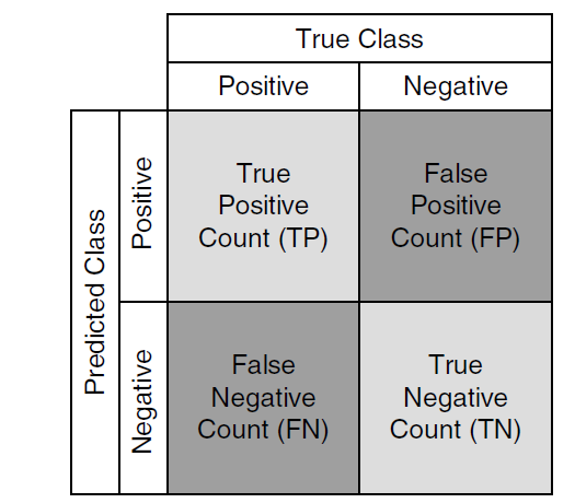
"Positives" or "Negatives" are defined as per the objective of the predictive model. For example, if the objective of the model is to predict whether the customer will "Buy" the product, the Number of possible "Buyers" will be counted as "positives" and "Non-Buyers" as "Negatives" Alternatively, if the objective of the model is to predict "Loan defaulters", then the Number of predicted Loan Defaulters will be classified as "Positive" result.

Performance Evaluation Metrics

In the field of machine learning, various evaluation metrics are employed to assess the performance of predictive models. Each metric provides unique insights into the model's behavior and can be used to measure different aspects of its effectiveness. Let's delve into the commonly used evaluation metrics:

1. Accuracy:

Accuracy is perhaps the most straightforward and commonly used evaluation metric. It measures the proportion of correct predictions made by the model out of the total number of predictions. In other words, it calculates the percentage of instances the model classified correctly.

Formula: Accuracy = (Number of Correct Predictions) / (Total Number of Predictions)

= (True Positives + True Negatives) / (Total Number of Predictions)

While accuracy is simple to interpret and understand, it may not be suitable for imbalanced datasets, where one class significantly outnumbers the other. In such cases, the accuracy metric can be misleading, as the model might perform well on the majority class but poorly on the minority class.

2. Precision and Recall:

Precision and recall are metrics commonly used in binary classification tasks, where the prediction is either positive or negative.

• Precision:

Precision measures the model's ability to correctly identify positive instances among the predicted positives. It calculates the proportion of true positive predictions out of the total predicted positive instances.

Formula: Precision = (True Positives) / (True Positives + False Positives)

High precision indicates that the model is accurate when it predicts positive instances, minimizing false positives. It is a crucial metric in scenarios where false positives can have significant consequences, such as in medical diagnoses or fraud detection.

• Recall:

Recall, also known as sensitivity or true positive rate, measures the model's ability to correctly identify positive instances among all actual positive instances. It calculates the proportion of true positive predictions out of the total actual positive instances.

Formula: Recall = (True Positives) / (True Positives + False Negatives)

High recall indicates that the model can identify most of the positive instances, minimizing false negatives. It is essential in situations where missing positive instances can have severe consequences, such as in disease diagnosis.

3. F1 Score:

The F1 Score is a metric that combines both precision and recall into a single value. It provides a balance between the two metrics, making it suitable for imbalanced datasets.

Formula: F1 Score = 2 * (Precision * Recall) / (Precision + Recall)

The F1 Score ranges from 0 to 1, where 1 indicates perfect precision and recall, and 0 means the worst performance. It is particularly useful when both false positives and false negatives need to be minimized.

4. ROC Curve and AUC:

The ROC (Receiver Operating Characteristic) Curve is a graphical representation of the model's performance across various classification thresholds. It plots the true positive rate (sensitivity) against the false positive rate (1 - specificity) as the threshold changes.

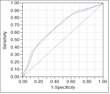
The ROC Curve helps assess the model's trade-off between sensitivity and specificity and its performance at different thresholds. A perfect model's ROC Curve would be a vertical line at true positive rate = 1 and false positive rate = 0.

AUC (Area Under the Curve):

The AUC is a single value that summarizes the overall performance of the ROC Curve. It calculates the area under the ROC Curve, representing the probability that the model will rank a randomly chosen positive instance higher than a randomly chosen negative instance.

The AUC value ranges from 0.5 to 1, where 0.5 indicates a model with no discrimination ability (random guessing), and 1 represents a perfect model with flawless predictions.

In conclusion, these commonly used evaluation metrics offer valuable insights into the performance of machine learning models. Each metric serves a specific purpose and helps data scientists and practitioners understand how well their models perform in different scenarios. Proper utilization of these metrics aids in the selection and optimization of models, ensuring their effectiveness in real-world applications.

Best Practices for Evaluating Model Performance

Evaluating model performance is akin to inspecting the precision of a finely tuned instrument – it's essential for ensuring accurate predictions and informed decision-making. In this segment, we'll delve into the best practices that pave the way for effective model evaluation, encompassing data splitting, handling imbalanced datasets, and the crucial role of cross-validation.

Splitting Data into Training, Validation, and Test Sets

Much like a sculptor carefully selects the right tools for each intricate detail, data scientists meticulously split their dataset into distinct subsets to ensure unbiased evaluation. This process involves dividing the dataset into three essential components:

Training Set: Building the Foundation

The training set is the realm where models learn patterns and relationships from data. Just as athletes train rigorously to excel, the training set is the model's arena to refine its predictive capabilities. It's crucial to feed the model enough diverse data to enable it to capture the underlying patterns effectively.

Validation Set: Fine-Tuning for Excellence

Similar to an artist scrutinizing their masterpiece before unveiling it, the validation set serves as the testing ground for model fine-tuning. Data scientists adjust hyperparameters and assess the model's performance on unseen data. This subset prevents overfitting and helps select the best-performing model configuration.

Test Set: The Ultimate Test

The test set is the grand stage where the model's performance is showcased. Just as athletes face the ultimate challenge in competition, the model confronts the test set to prove its prowess. The data in the test set should remain entirely unseen during model development to ensure an accurate assessment of its generalization capabilities.

Dealing with Imbalanced Datasets: Achieving Balance

In the realm of modeling, imbalanced datasets are like uneven terrain for athletes. They can skew model performance, favoring the majority class. To address this challenge, data scientists adopt various strategies:

• Resampling: Balancing class distribution by either oversampling the minority class or undersampling the majority class.
• Synthetic Data Generation: Creating artificial examples for the minority class using methods like SMOTE (Synthetic Minority Over-sampling Technique).
• Metrics Selection: Prioritizing metrics like precision, recall, and F1 score that are more robust in imbalanced scenarios.

The Importance of Cross-Validation: A Holistic Assessment

Cross-validation serves as the model's comprehensive performance appraisal, much like a panel of judges in a competition. Techniques like K-Fold and Stratified Cross-Validation ensure a holistic evaluation:

• K-Fold Cross-Validation: Divides the dataset into K subsets, iteratively training on K-1 subsets and validating on the remaining one.
• Stratified Cross-Validation: Maintains class distribution balance in each fold, crucial for imbalanced datasets.

Cross-validation addresses concerns about data variability, ensuring that a model's performance is consistent and not a result of chance. Moreover, it aids in hyperparameter tuning, leading to a more robust and accurate model. We will discuss these in detail the following sections.

Cross-Validation Techniques

Cross-validation is a critical technique in machine learning for assessing a model's performance on unseen data while avoiding overfitting. It involves partitioning the dataset into subsets for training and validation, allowing for a more robust evaluation of the model's generalization capabilities. Here, we'll delve into three popular cross-validation techniques: K-Fold Cross-Validation, Stratified Cross-Validation, and Leave-One-Out Cross-Validation.

K-Fold Cross-Validation

K-Fold Cross-Validation is like a chef carefully sampling their culinary creation from various portions to ensure consistency. The dataset is divided into K equally-sized folds. The model is trained K times, each time using K-1 folds for training and the remaining fold for validation. This rotation of folds ensures that each data point is part of the validation set once and the training set K-1 times.

K-Fold Cross-Validation provides a more reliable estimate of a model's performance on unseen data than a single train-test split. The final evaluation metric is often the average performance across all K iterations. This technique is particularly useful when the dataset is not excessively large, as it requires training K models.

Stratified Cross-Validation

Imagine organizing a party where you ensure a proportional representation of different age groups to make everyone feel included. Stratified Cross-Validation does something similar by preserving the class distribution in each fold. This is crucial when dealing with imbalanced datasets, where one class significantly outnumbers the other.

In Stratified Cross-Validation, each fold contains a representative proportion of each class, ensuring that rare classes are not left out. This technique enhances the reliability of the model's evaluation, especially in scenarios where class imbalance is prevalent.

Leave-One-Out Cross-Validation

Leave-One-Out Cross-Validation (LOOCV) is like testing the resilience of a bridge by removing one brick at a time to see if it still stands. In LOOCV, each data point serves as a validation set, while the remaining data points are used for training. This means that you create as many folds as there are data points, leading to an exhaustive evaluation.

LOOCV provides an accurate estimate of the model's performance, but it's computationally intensive, especially for large datasets, as it requires training a model for each data point. Despite its resource demand, LOOCV is particularly useful when dealing with limited datasets, where every data point is valuable.

Choosing the Right Technique

The choice of cross-validation technique depends on various factors:

• Dataset Size: For larger datasets, K-Fold Cross-Validation is efficient, while LOOCV is suitable for smaller datasets.
• Imbalanced Datasets: Stratified Cross-Validation is essential when dealing with imbalanced datasets to ensure fair representation of all classes.
• Computational Resources: LOOCV demands more computational resources due to its exhaustive nature, whereas K-Fold Cross-Validation is less resource-intensive.
• Bias-Variance Tradeoff: LOOCV tends to have a lower bias but higher variance due to training multiple models, while K-Fold Cross-Validation strikes a balance between bias and variance.

Cross-validation techniques are powerful tools for assessing a model's performance and generalization ability. K-Fold Cross-Validation, Stratified Cross-Validation, and Leave-One-Out Cross-Validation offer different advantages and are chosen based on factors like dataset size, class distribution, and computational resources. By employing these techniques, data scientists ensure that their models are well-evaluated, leading to better model selection, hyperparameter tuning, and ultimately, more accurate predictions in real-world applications.

The Bias-Variance Tradeoff

In the realm of machine learning, the bias-variance tradeoff is a fundamental concept that underpins model performance. It highlights the delicate balance between two essential sources of error in models: bias and variance. Mastering this tradeoff is crucial for creating models that generalize well to unseen data.

Understanding Bias and Variance

Imagine training a model to predict a target value. Bias refers to the error introduced by approximating a real-world problem, which may be complex, by a simplified model. A model with high bias oversimplifies the problem and is likely to make systematic errors regardless of the training data.

On the other hand, variance pertains to the model's sensitivity to fluctuations in the training dataset. A model with high variance fits the training data too closely, capturing noise and leading to poor generalization on unseen data. It essentially overfits the training data.

Impact on Model Performance

To comprehend the impact of bias and variance on model performance, consider an archer aiming at a target. If the archer consistently hits off-center but close to each other, it's a high bias, low variance situation. The archer is biased but not very sensitive to changes. Conversely, if the arrows are scattered all over, it's a high variance, low bias scenario.

High Bias, Low Variance: The model is systematically wrong but consistently so. It fails to capture the complexities of the data. The model might overlook important patterns.

High Variance, Low Bias: The model is sensitive to noise in the training data. It fits the data perfectly but performs poorly on new data. It essentially memorizes the training data.

Achieving the Optimal Balance

Striking the right balance between bias and variance is the ultimate goal in model development. The objective is to create a model that performs well on both the training data and unseen data. Achieving this balance enhances the model's generalization ability.

Bias-Variance Tradeoff Strategies:

1. Model Complexity: Increasing model complexity reduces bias but increases variance. Simplifying the model reduces variance but increases bias.
2. Regularization: Techniques like Lasso and Ridge regression introduce penalties that discourage extreme parameter values. They reduce model complexity, mitigating variance.
3. Ensemble Methods: Combining multiple models can balance bias and variance. Techniques like bagging and boosting help in achieving this balance.
4. Feature Selection: Removing irrelevant features can reduce variance caused by noise in the data.
5. Training Data Size: More data often reduces variance by providing a more representative sample of the underlying distribution.
6. Hyperparameter Tuning: Fine-tuning hyperparameters can help find the optimal balance. For example, adjusting the learning rate in gradient boosting can influence bias and variance.

The bias-variance tradeoff serves as a guiding principle in machine learning. Understanding this tradeoff is pivotal for developing models that generalize effectively to new data. High bias leads to systematic errors, while high variance leads to overfitting. Achieving the optimal balance requires careful consideration of model complexity, regularization, ensemble methods, feature selection, data size, and hyperparameter tuning. Striking the right balance empowers data scientists to create models that exhibit robust performance across a range of scenarios, making them valuable tools for making accurate predictions and data-driven decisions.

Hyperparameter Tuning: Unveiling the Essence of Model Optimization

In the labyrinth of machine learning, hyperparameter tuning emerges as a beacon guiding model optimization. Just as a conductor refines an orchestra's performance by adjusting instruments, hyperparameter tuning fine-tunes a model's parameters to achieve peak efficiency. This exploration into hyperparameter tuning will unveil its importance, delve into the showdown between Grid Search and Random Search, and explore other potent hyperparameter optimization techniques.

Importance of Hyperparameter Tuning

Imagine a painter blending colors to create the perfect shade. Hyperparameter tuning is akin to finding the right mix of parameters to orchestrate a model's best performance. Hyperparameters influence a model's learning process, affecting its convergence, accuracy, and generalization.

Key Aspects of Hyperparameter Tuning:

1. Overfitting and Underfitting: Optimal hyperparameters strike a balance between overfitting (high variance) and underfitting (high bias).
2. Efficiency: Proper hyperparameters accelerate a model's convergence, reducing the time and resources required for training.
3. Generalization: Well-tuned hyperparameters enhance a model's ability to generalize predictions to unseen data.
4. Model Complexity: Hyperparameters influence a model's complexity, impacting its capability to capture intricate patterns.

Grid Search vs. Random Search

The battle of giants: Grid Search and Random Search are two popular hyperparameter tuning approaches.

Grid Search is systematic, akin to a detective meticulously examining each clue. It defines ranges for hyperparameters and tests all possible combinations. Grid Search's thoroughness guarantees that no stone is left unturned. However, it can be computationally expensive and inefficient, especially when hyperparameter spaces are vast.

Random Search, the daredevil, randomly samples hyperparameters from predefined ranges. It's less exhaustive than Grid Search, but often more efficient. Random Search exploits the notion that even a few well-chosen random combinations can lead to impressive results.

Other Hyperparameter Optimization Techniques

1. Bayesian Optimization: This method models the objective function to predict promising hyperparameter configurations. It adapts its search based on past trials, making it efficient for complex functions.
2. Genetic Algorithms: Inspired by evolution, Genetic Algorithms evolve a population of hyperparameter configurations over multiple generations, selecting the best performers.
3. Particle Swarm Optimization: This technique mimics the social behavior of birds flocking or fish schooling to find optimal hyperparameters.
4. Gradient-Based Optimization: These methods employ gradients to update hyperparameters iteratively, optimizing performance.
5. Automated Hyperparameter Tuning Tools: Libraries like Optuna and Hyperopt automate hyperparameter tuning, easing the burden on data scientists.

Choosing the Right Approach

The choice between Grid Search, Random Search, or other techniques depends on factors like dataset size, computational resources, and complexity of the model. Bayesian Optimization and Genetic Algorithms are favored for complex functions, while simpler models might benefit from Grid or Random Search.

Hyperparameter tuning is the compass guiding machine learning models to their true potential. Its significance lies in the delicate balance it achieves between model performance, efficiency, and generalization. The choice between Grid Search and Random Search depends on the problem's complexity and computational constraints. Moreover, other techniques like Bayesian Optimization, Genetic Algorithms, and automated tools further enrich the arsenal of hyperparameter optimization. By mastering hyperparameter tuning, data scientists empower models to shine brightly, rendering accurate predictions and invaluable insights for diverse real-world applications.

Conclusion: Elevating Model Evaluation

Best practices for evaluating model performance are the compass that guides data scientists in the pursuit of accurate predictions. Splitting data into training, validation, and test sets ensures fair evaluation, while strategies for imbalanced datasets empower models to tackle real-world scenarios. The pivotal role of cross-validation ensures a comprehensive assessment, enhancing model generalization and contributing to informed decision-making. By adhering to these practices, data scientists equip themselves with the tools to extract reliable insights from data, shaping the landscape of effective machine learning.